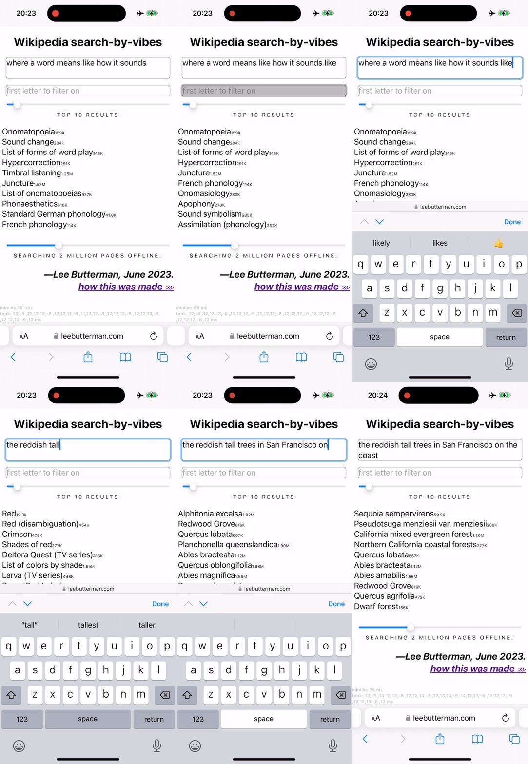
Wikipedia search-by-vibes through millions of pages offline
What is this?
Check it out! https://leebutterman.com/wikipedia-search-by-vibes/

Anatomy of a realtime offline in-browser embedding search engine
This is an exploration of several proof points:
- Vector search can be performant without being complicated
- use Product Quantization and linear scans, even for a faceted search
- ONNX Runtime is powerful
- handwritten opcodes to avoid losses in PyTorch translation
- Browsers are fast enough for realtime inference
- use WASM and (maybe some day) WebGPU
Specifically, the facet that we are searching on is the first letter of the title: to search through our dataset by vector similarity for some columns (the embedding of the body text) and equality for other columns (first letter of title) is tantamount to a full-fledged database query use case.
The constraints of an offline browser-based app inspire significant architectural choices: the embeddings have to be very small, the embedding model has to be open source, and the embedding model should be relatively lightweight in size and compute. Generally, lightweight means under 100MB, in 2023.
Data
English Wikipedia, via all-minilm-l6-v2 averaged embeddings
The dataset is English Wikipedia, embedded with the model all-minilm-l6-v2. There are 6M documents, and we average the embeddings across the chunks of the page. We order pages by reverse page length, putting longer pages first, so that as we progressively load more of the database, we load the pages with the most human effort in them first.
The dimensions of the embedding is 384. With 32-bit floats, our dataset is of size 6M * 384 * 4 = 9GB, and we can store 64k embeddings in 96MB. This encoding is less efficient than we’d like!
Product Quantization
To quantize a single embedding, we make (one or more) palettes of interesting floating point numbers, and each floating point input becomes an index into a palette. Often these palettes have under 256 values, so that each palette index is at most a byte. Sometimes these palettes are implicit, like the number line from -127 to 127 or the number line from 0 to 255, shifted and stretched somehow and only the shifting and stretching parameters get stored. Sometimes these palettes are explicit, like 256 numbers stored one after the other. Product Quantization’s palettization is explicit.
How many palettes is the right number?
At minimum, we need one palette. If we would transform our 384-dimension embedding into 384 indices, we would have a palette of size 256 * 4 = 1K, and our dataset would be of size 6M * 384 = 2.25GB, and we could store 256K embeddings in 96MB. This encoding is better and still less efficient than we’d like!
[Sentence 1]                         [Sentence 2]                         [Sentence 3]

     |                                     |                                    |
     v                                     v                                    v

|------------------------------------------------------------------------------------|
|                                   embedding model                                  |
|------------------------------------------------------------------------------------|

     |                                     |                                    |
     v                                     v                                    v


[0.8][0.3][-.2][0.6][-.5][…]     [0.7][0.2][-.3][0.5][-.6][…]      [0.4][-.5][0.8][0.9][0.1][…]

  |    |    |    |                 |    |    |    |                  |    |    |    |
  |--- | -- | -- | -------------------- | -- | -- | -----------------/    |    |    |
  |    |    |    |                      |    |    |                       |    |    |
  |    |--- | -- | ------------------------- | -- | ----------------------/    |    |
  |         |    |        |                  |    |                            |    |
  |         |--- | ------------------------------ | ---------------------------/    |
  |              |        |                       |     |                           |
  |               \-----------------------------------------------------------------/
  |                       |                             |                       |
  |                       |                             |                       |
  v                       v                             v                       v

-1 -xxxXXxxx- +1       -1 -xxXXXXXx- +1            -1 -XXXXXXXX- +1       -1 -xxxxXxxX- +1

       |                       |                          |                      |
       |                       |                          |                      |
       |                       |                          |                      |
       v                       v                          v                      v

-(X)--(X)(X)--(X)-     --(X)(X)-(X)(X)--           -(X)-(X)-(X)-(X)-      ---(X)(X)-(X)(X)-
We could have a different palette for every dimension of our embedding. This amounts to 384 palettes (which is 384K, very small), but we still have a dataset that is the same size.
What if we have a palette that represents a 2d point? If we take the product of two dimensions in our embedding, and perform quantization to find the 256 best 2d points, then we will have 192 indices, for a 2x space saving! This is Product Quantization .
[Sentence 1]                         [Sentence 2]                         [Sentence 3]

     |                                     |                                    |
     v                                     v                                    v

|------------------------------------------------------------------------------------|
|                                   embedding model                                  |
|------------------------------------------------------------------------------------|

     |                                     |                                    |
     v                                     v                                    v


[0.8][0.3][-.2][0.6][-.5][…]     [0.7][0.2][-.3][0.5][-.6][…]      [0.4][-.5][0.8][0.9][0.1][…]

    \/        \/                     \/        \/                      \/        \/
    |         |                      |         |                       |         |
    |-------- | ------------------------------ | ----------------------/         |
    |         |                                |                                 |
    |         |--------------|---------------------------------------------------/
    |                        |
    |                        |
    |                        |
    v                        v

       +1
       | ...
       |x@@.                     +1
       |@@@x                 ....|
      x|X@@x                 .@@X|x.
-1 ----+---- +1               x@@|X.
     xx|X                     .Xx|.
    ..X|                  -1 ----+---- +1
    .. |                         |xXx
       |                         | .
       -1                        |
                                 |
                                 -1

      |                          |
      |                          |
      |                          |
      v                          v


       +1                         +1
       |                          |
       | (X)                  (X) |
       |    (X)                   |(X)
       |(X)                    (X)|
-1 ----+---- +1            -1 ----+---- +1
    (X)|                          |(X)
       |                          |
       |                          |
       |                          |
       -1                         -1
Note that we can use more than 2 dimensions as well. For example, we can use an 8-dimensional point, which will give us 48 indices to 8-dimensional points, for a palette of the same 384K size, but a dataset of size 6M * 48 = 288M, and we can store 2M embeddings in 96MB! This level of quantization is what we use, and we can evaluate precision and recall for any level of quantization.
Product Quantization search
Crucially, we can search in the compressed domain!
If we have n dimensions, we can group this into n/2 2-d points. We can take our palette of 2-d points, and compute the distance from each 2-d point to the corresponding 2-d point in the query. Now we have a palette of distances that we can index into. We can do n/2 index lookups to fetch distances and add the distances up. This is less than half of the work of generating the full n-dimensional point, computing the distance across each dimension, and adding all of those up.
In our 8-dimensional points that we use in production, this is an eighth of the work of dealing with uncompressed embeddings.
Arrow as data exchange format
Data movement and transformation get expensive. Ideally we will serialize our compressed embeddings in a format that can be immediately used.
Arrow is designed for exactly this. We can store an Arrow table of embeddings and page titles, and we will use columnar storage, and have a 2-d array of our palette indexes, and a 1-d array of our titles as strings, and we will not spend any time on parsing or loading apart from copying the bits into place.
Because the Arrow array format only stores one-dimensional data, and because we have 48 dimensions of embedding data, and because we do not want to store embedding data wrapped in another data format, we need two separate schemas, one for the metadata (with a hundred thousand rows each), and one for the embeddings (with a hundred thousand * 48 rows each), and we reshape the embeddings at load time.
Note that safetensors follows this design principle.
Contrast this with JSON, where we will be serializing an array of 48 elements to an unknown number of ASCII characters, which requires an intricate loading step. Contrast this with Protocol Buffers, which use base 128 variable-width integers for less-than-32-bit-wide integers: this integer format is not well supported by current compute kernels.
Code
Parsing Wikipedia entries via OLM’s wikipedia dataset + mwparserfromhell
The most capable parser of Wiki markup is the mediawiki parser from hell. OLM has a Dataset in Huggingface that will fetch the latest data dump for a particular language’s wikipedia, and parse that into rows of text with titles and such (this dataset is mostly code, that we will need to trust running, versus mostly data in innocuous serialization formats).
The parsing happens across all cores of the one machine that it runs on. Modern machines have dozens of cores, so this is perfect for the under 100M-document regime of English Wikipedia (currently 6M pages).
Embedding via all-minilm-l6v2
There are a lot of sentence transformers to choose from! There is a leaderboard of sentence embeddings: https://huggingface.co/blog/mteb
A performant and lightweight embedding model for English is all-minilm-l6-v2. Queries and documents embed into the same space, and the performance is good enough to run off-the-shelf. There are 8-bit quantizations of all-minilm-l6-v2 available, to run in Javascript in the browser via ONNX and transformers.js. At 22M parameters, this model is very lightweight.
The context window is much shorter than the average page length, trained on 128-token sequences. We thus chunk the page, and average the embeddings of each chunk, to get an average page embedding.
Faceted vector search via pq.js and linear scans
There are a lot of complex indexing schemes. For only millions of documents, running locally, we do not need any of them.
We want to end up with the top dozen distances from a particular point.
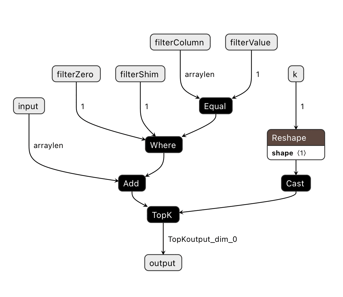
We can take an array of ten million distances, a facet column of ten million values to filter on, a facet value to match, and we can add either 0 or Infinity to the distances based on the facet value equality and find the top hundred in under 10ms on a modern phone. This is filtered-topk in pq.js.
class FilteredTopKModel(nn.Module):
    def __init__(self):
        super(FilteredTopKModel, self).__init__()

    def forward(self, x, filterColumn, filterValue, z, shim, k):
        (topk_values, topk_indices) = torch.topk(
            x + torch.where(filterColumn == filterValue, z, shim) ,
            k.to(torch.int64),
            largest=False)
        return topk_indices
We can export this PyTorch module as an ONNX model, and the control flow is:

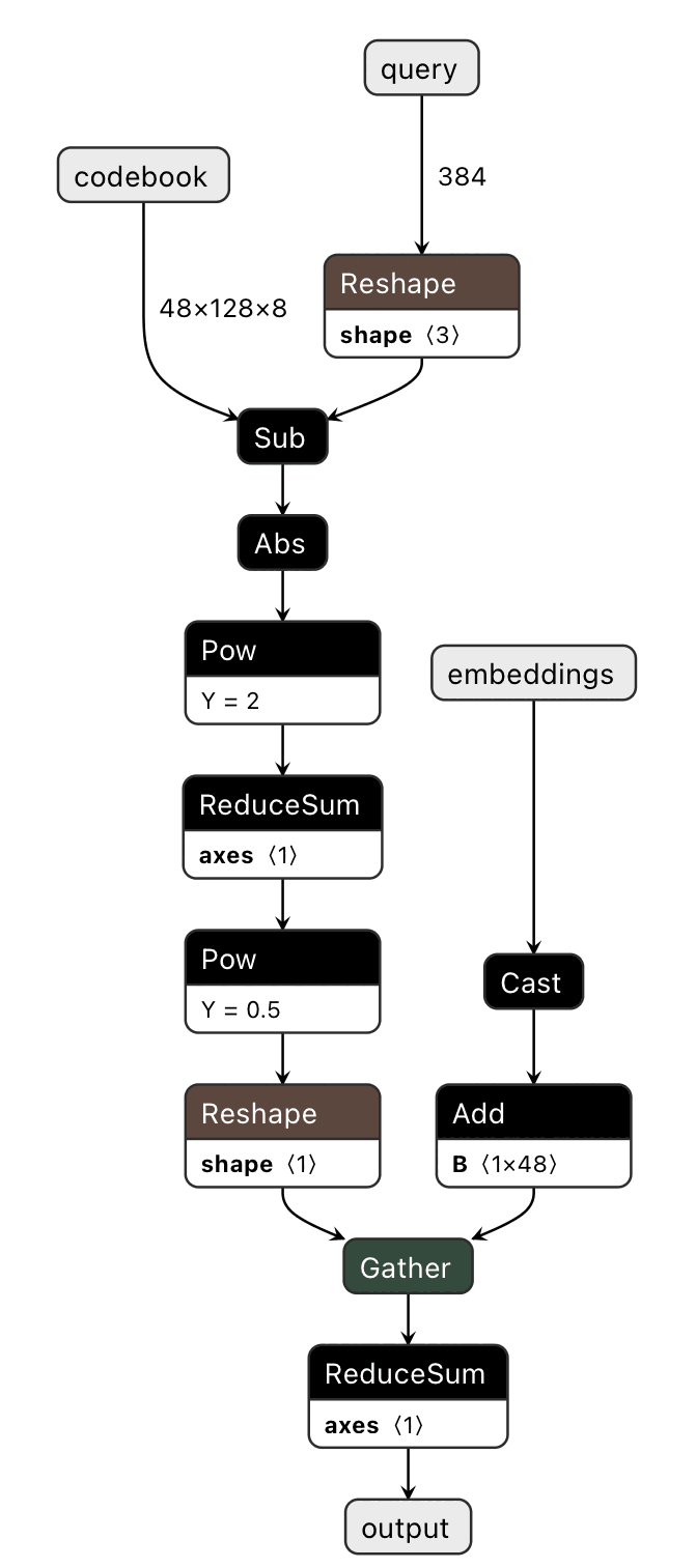
Now we need to compute the distances. We can write compute distances of embeddings compressed with product quantization in PyTorch relatively straightforwardly:
class PQSmolDistModel(nn.Module):
    def __init__(self, subspaceCount, subspaceDim, codewordCount):
        super(PQSmolDistModel, self).__init__()
        self.subspaceCount = subspaceCount
        self.subspaceDim = subspaceDim
        self.codewordCount = codewordCount

    def forward(self, query, codewords, embeddings):
        starttime = time.time()
        dtable = torch.linalg.norm(
            codewords - torch.reshape(query, (self.subspaceCount, 1, self.subspaceDim)),
            axis=2
        )
        dists = torch.sum(dtable.reshape(-1)[
            embeddings.to(torch.int32) +
            torch.arange(self.subspaceCount, dtype=torch.int32).unsqueeze(0) * self.codewordCount
        ], dim=1)
        endtime = time.time()
        print(f"timing {endtime - starttime}")
        return dists
where we have subspaceCount different palettes, each holding codewordCount different subspaceDim-dimensional points.

However, the indexing is a bit of a kludge.
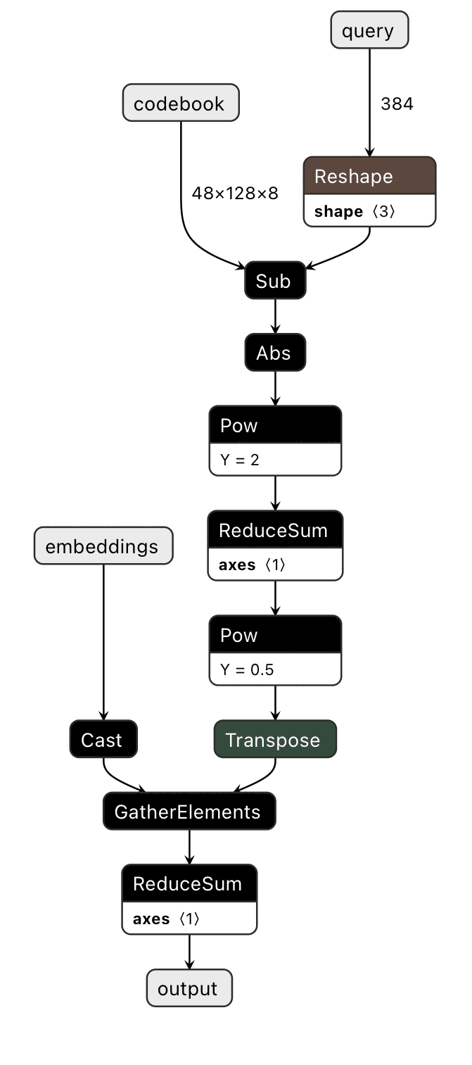
There is a GatherElements opcode in ONNX that does exactly what we need. We need to replace a few nodes and this is well supported by the ecosystem using tools like ONNX-modifier, a graphical tool to add and delete elements of the dataflow graph of an exported ONNX model.
By taking the multiple steps of indexing and replacing them with a single opcode that does the correct operation, distance computation is roughly 4x faster.

Note that we do not have a fixed size of embeddings to compute distance for: we can stream distances from a query to a subset of embeddings, and when enough time has passed, we can run our top-k computation and update our query results based on our new distances. This is only feasible because all of the embeddings are local and the latency to the search infrastructure is effectively 0ms.
Also note that we want this interactive. We want to manipulate the UI and see results happening in 100-300ms. We can run minilm in under 100ms (often in under 15ms depending on the edge device), we can run a distance computation over 100k embeddings in about 10ms, and we can choose an update interval at which point we will stop running distance computation and start running top-k on our results so far, for updates in our React UI. This gives us a high degree of interactivity while allowing for long-running computation. Note that in general longer articles have had more attention and interest given to them while writing, and are often better matches for the search query than any of the numerous stub articles: this means that by ordering our dataset from longest to shortest article, and by streaming results in, most of the final top search results land early.
Also note that by computing distances globally and then filtering and computing the top k, we can select different facet values or different number of search results for the same query and those return with just a run of the filtering, which is under 10ms, which feels instant.
Let me know what you think 🙂
Lots of the library functions in the full Wikipedia search app should migrate into reusable pq.js components. A lot of the ONNX shapes are pre-baked, so it would be useful to support different quantization levels and different embedding dimensions. Give a shout!